Navigating Linear Regression in Machine Learning

Linear regression is a fundamental concept in machine learning, widely used for predicting continuous values based on input features. It is a simple yet powerful technique that forms the basis for more complex algorithms in the field. In this article, we will delve into the details of linear regression, its assumptions, implementation, and evaluation.

What is Linear Regression?

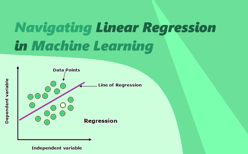
Linear regression is a supervised learning algorithm used for predicting a continuous target variable based on one or more input features. It assumes a linear relationship between the input variables and the output variable. The algorithm aims to find the best-fit line that minimizes the difference between the predicted and actual values.

Suggested: Exploring Gaussian Mixture Model (GMM) Clustering: A Detailed Analysis

Assumptions of Linear Regression

Before applying linear regression, it is important to understand the assumptions associated with it:

1. Linearity: The relationship between the input and output variables should be linear.
2. Independence: The observations should be independent of each other.
3. Homoscedasticity: The variance of the errors should be constant across all levels of the input variables.
4. Normality: The errors should follow a normal distribution.

Implementation of Linear Regression

The implementation of linear regression involves the following steps:

1. Data Preprocessing: Clean the data by handling missing values, outliers, and categorical variables.
2. Splitting the Data: Divide the dataset into training and testing sets.
3. Feature Scaling: Normalize or standardize the input features if necessary.
4. Model Training: Fit the linear regression model to the training data.
5. Model Evaluation: Assess the performance of the model using evaluation metrics such as mean squared error (MSE) or R-squared.

Evaluation of Linear Regression

There are several evaluation metrics used to assess the performance of a linear regression model:

• Mean Squared Error (MSE): It measures the average squared difference between the predicted and actual values.
• R-squared: It represents the proportion of the variance in the target variable that can be explained by the input variables.
• Root Mean Squared Error (RMSE): It is the square root of the MSE and provides a more interpretable measure of the model’s performance.
• Adjusted R-squared: It adjusts the R-squared value based on the number of input variables and the sample size.

Advantages and Limitations of Linear Regression

Linear regression has several advantages:

• It is easy to understand and interpret.
• It provides a good baseline model for comparison with more complex algorithms.
• It can handle both numerical and categorical input variables.

However, linear regression also has certain limitations:

• It assumes a linear relationship between the input and output variables, which may not always hold true.
• It is sensitive to outliers and can be influenced by them.
• It may not perform well when the assumptions of linearity, independence, homoscedasticity, and normality are violated.

Types of Linear Regression

Simple Linear Regression

Simple linear regression is the most basic form of linear regression. It involves only one independent variable and one dependent variable. The goal is to find the best-fitting line that represents the relationship between the two variables. The equation of a simple linear regression model is:

y = β₀ + β₁x + ε

where y is the dependent variable, x is the independent variable, β₀ is the y-intercept, β₁ is the slope of the line, and ε is the error term.

Multiple Linear Regression

Multiple linear regression extends the concept of simple linear regression by including multiple independent variables. It is used when there is more than one factor that can affect the dependent variable. The equation of a multiple linear regression model is:

y = β₀ + β₁x₁ + β₂x₂ + … + β_nx_n + ε

where y is the dependent variable, x₁, x₂, …, x_n are the independent variables, β₀ is the y-intercept, β₁, β₂, …, β_n are the slopes of the lines, and ε is the error term.

Polynomial Regression

Polynomial regression is a type of regression analysis in which the relationship between the independent variable(s) and the dependent variable is modeled as an nth degree polynomial. It is used when the relationship between the variables is not linear. The equation of a polynomial regression model is:

y = β₀ + β₁x + β₂x² + … + β_nxⁿ + ε

where y is the dependent variable, x is the independent variable, β₀ is the y-intercept, β₁, β₂, …, β_n are the coefficients of the polynomial terms, and ε is the error term.

Ridge Regression

Ridge regression is a regularization technique used to overcome the problem of multicollinearity in multiple linear regression. Multicollinearity occurs when there is a high correlation between independent variables, which can lead to unstable and unreliable estimates of the regression coefficients. Ridge regression adds a penalty term to the least squares objective function, which helps to reduce the impact of multicollinearity. The equation of a ridge regression model is similar to that of multiple linear regression, but with an additional penalty term:

y = β₀ + β₁x₁ + β₂x₂ + … + β_nx_n + λΣβ_i² + ε

where y is the dependent variable, x₁, x₂, …, x_n are the independent variables, β₀ is the y-intercept, β₁, β₂, …, β_n are the slopes of the lines, λ is the regularization parameter, Σβ_i² is the sum of squared regression coefficients, and ε is the error term.

Lasso Regression

Lasso regression is another regularization technique used to overcome the problem of multicollinearity in multiple linear regression. It is similar to ridge regression, but with a different penalty term. Lasso regression adds the absolute values of the regression coefficients to the least squares objective function, which encourages sparsity in the model. This means that some of the coefficients may be exactly zero, effectively removing the corresponding independent variables from the model. The equation of a lasso regression model is:

y = β₀ + β₁x₁ + β₂x₂ + … + β_nx_n + λΣ|β_i| + ε

where y is the dependent variable, x₁, x₂, …, x_n are the independent variables, β₀ is the y-intercept, β₁, β₂, …, β_n are the slopes of the lines, λ is the regularization parameter, Σ|β_i| is the sum of absolute values of the regression coefficients, and ε is the error term.

Conclusion

Linear regression is a versatile algorithm that forms the foundation of many machine learning techniques. It is important to understand its assumptions, implementation steps, and evaluation metrics to effectively apply it to real-world problems. By considering its advantages and limitations, we can make informed decisions about when and how to use linear regression in machine learning projects.